單擺和雙擺模擬?

單擺模擬?

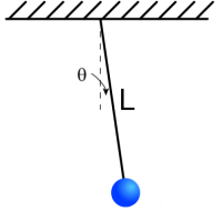
由一根不可伸長、質量不計的繩子，上端固定，下端系一質點，這樣的裝置叫做單擺。

單擺裝置示意圖

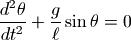
根據牛頓力學定律，我們可以列出如下微分方程：

${d^2\theta\over dt^2}+{g\over \ell} \sin\theta=0$

其中 $\theta$ 為單擺的擺角， $\ell$ 為單擺的長度， g為重力加速度。

此微分方程的符號解無法直接求出，因此只能調用odeint對其求數值解。

odeint函數的調用參數如下：

odeint(func, y0, t, ...)

其中func是一個Python的函數對象，用來計算微分方程組中每個未知函數的導數，y0為微分方程組中每個未知函數的初始值，t為需要進行數值求解的時間點。它返回的是一個二維數組result，其第0軸的長度為t的長度，第1軸的長度為變量的個數，因此 result[:, i] 為第i個未知函數的解。

計算微分的func函數的調用參數為： func(y, t)，其中y是一個數組，為每個未知函數在t時刻的值，而func的返回值也是數組，它為每個未知函數在t時刻的導數。

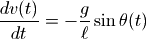
odeint要求每個微分方程只包含一階導數，因此我們需要對前面的微分方程做如下的變形：

${d\theta(t)\over dt} = v(t)$

${dv(t)\over dt} = -{g\over \ell} \sin\theta(t)$

下面是利用odeint計算單擺軌跡的程序：

# -*- coding: utf-8 -*-

from math import sin
import numpy as np
from scipy.integrate import odeint

g = 9.8

def pendulum_equations(w, t, l):
    th, v = w
    dth = v
    dv  = - g/l * sin(th)
    return dth, dv
    
if __name__ == "__main__":
    import pylab as pl
    t = np.arange(0, 10, 0.01)
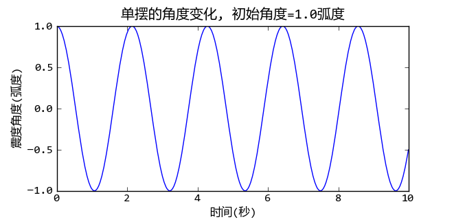
    track = odeint(pendulum_equations, (1.0, 0), t, args=(1.0,))
    pl.plot(t, track[:, 0])
    pl.title(u"單擺的角度變化, 初始角度=1.0弧度")
    pl.xlabel(u"時間(秒)")
    pl.ylabel(u"震度角度(弧度)")
    pl.show()

odeint函數還有一個關鍵字參數args，其值為一個組元，這些值都會作為額外的參數傳遞給func函數。程序使用這種方式將單擺的長度傳遞給pendulum_equations函數。

初始角度為1弧度的單擺擺動角度和時間的關系

計算擺動周期?

高中物理課介紹過當最大擺動角度很小時，單擺的擺動周期可以使用如下公式計算：

$T_0 = 2\pi\sqrt{\frac{\ell}{g}}$

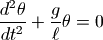
這是因為當 $\theta << 1$ 時， $\sin\theta\approx\theta$ ，這樣微分方程就變成了：

${d^2\theta\over dt^2}+{g\over \ell}\theta=0$

此微分方程的解是一個簡諧震動方程，很容易計算其擺動周期。但是當初始擺角增大時，上述的近似處理會帶來無法忽視的誤差。下面讓我們來看看如何用數值計算的方法求出單擺在任意初始擺角時的擺動周期。

要計算擺動周期只需要計算從最大擺角到0擺角所需的時間，擺動周期是此時間的4倍。為了計算出這個時間值，首先需要定義一個函數pendulum_th計算任意時刻的擺角：

def pendulum_th(t, l, th0):
    track = odeint(pendulum_equations, (th0, 0), [0, t], args=(l,))
    return track[-1, 0]

pendulum_th函數計算長度為l初始角度為th0的單擺在時刻t的擺角。此函數仍然使用odeint進行微分方程組求解，只是我們只需要計算時刻t的擺角，因此傳遞給odeint的時間序列為[0, t]。 odeint內部會對時間進行細分，保證最終的解是正確的。

接下來只需要找到第一個時pendulum_th的結果為0的時間即可。這相當于對pendulum_th函數求解，可以使用 scipy.optimize.fsolve 函數對這種非線性方程進行求解。

def pendulum_period(l, th0):
    t0 = 2*np.pi*sqrt( l/g ) / 4
    t = fsolve( pendulum_th, t0, args = (l, th0) )
    return t*4

和odeint一樣，我們通過fsolve的args關鍵字參數將額外的參數傳遞給pendulum_th函數。fsolve求解時需要一個初始值盡量接近真實的解，用小角度單擺的周期的1/4作為這個初始值是一個很不錯的選擇。下面利用pendulum_period函數計算出初始擺動角度從0到90度的擺動周期：

ths = np.arange(0, np.pi/2.0, 0.01)
periods = [pendulum_period(1, th) for th in ths]

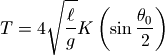
為了驗證fsolve求解擺動周期的正確性，我從維基百科中找到擺動周期的精確解：

$T = 4\sqrt{\ell\over g}K\left(\sin{\theta_0\over 2} \right)$

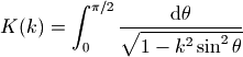
其中的函數K為第一類完全橢圓積分函數，其定義如下：

$K(k) = \int_0^{\pi/2} \frac{{\rm{d}}\theta}{\sqrt{1-k^2 \sin^2\theta}}$

我們可以用 scipy.special.ellipk 來計算此函數的值：

periods2 = 4*sqrt(1.0/g)*ellipk(np.sin(ths/2)**2)

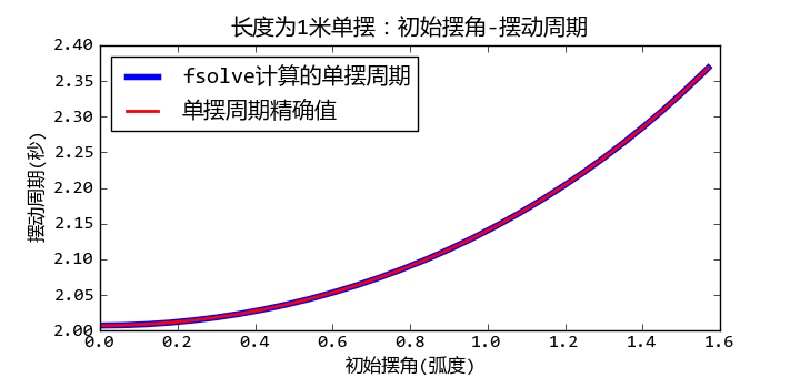
下圖比較兩種計算方法，我們看到其結果是完全一致的：

單擺的擺動周期和初始角度的關系

完整的程序請參見： 單擺擺動周期的計算

雙擺模擬?

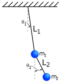
接下來讓我們來看看如何對雙擺系統進行模擬。雙擺系統的如下圖所示，

雙擺裝置示意圖

兩根長度為L1和L2的無質量的細棒的頂端有質量分別為m1和m2的兩個球，初始角度為 $\theta_1$ 和 $\theta_2$ ，要求計算從此初始狀態釋放之后的兩個球的運動軌跡。

公式推導?

本節首先介紹如何利用拉格朗日力學獲得雙擺系統的微分方程組。

拉格朗日力學(摘自維基百科)

拉格朗日力學是分析力學中的一種。於 1788 年由拉格朗日所創立，拉格朗日力學是對經典力學的一種的新的理論表述。

經典力學最初的表述形式由牛頓建立，它著重於分析位移，速度，加速度，力等矢量間的關系，又稱為矢量力學。拉格朗日引入了廣義坐標的概念，又運用達朗貝爾原理，求得與牛頓第二定律等價的拉格朗日方程。不僅如此，拉格朗日方程具有更普遍的意義，適用范圍更廣泛。還有，選取恰當的廣義坐標，可以大大地簡化拉格朗日方程的求解過程。

假設桿L1連接的球體的坐標為x1和y1，桿L2連接的球體的坐標為x2和y2，那么x1,y1,x2,y2和兩個角度之間有如下關系：

$x_1 &= L_1 \sin(\theta_1)$

$y_1 &= -L_1 \cos(\theta_1)$

$x_2 &= L_1 \sin(\theta_1) + L_2 \sin(\theta_2)$

$y_2 &= -L_1 \cos(\theta_1) - L_2 \cos(\theta_2)$

根據拉格朗日量的公式：

$\mathcal{L}=T-V$

其中T為系統的動能，V為系統的勢能，可以得到如下公式：

$\mathcal{L} = \frac{m_1}{2} ( {\dot x_1}^2 + {\dot y_1}^2 ) + \frac{m_2}{2} ( {\dot x_2}^2 + {\dot y_2}^2 ) - m_1 g y_1 - m_2 g y_2$

其中正號的項目為兩個小球的動能，符號的項目為兩個小球的勢能。

將前面的坐標和角度之間的關系公式帶入之后整理可得：

$\mathcal{L} = \frac{m_1+m_2}{2} L_1^2 {\dot \theta_1}^2 + \frac{m_2}{2} L_2^2 {\dot \theta_2}^2 + m_2 L_1 L_2 {\dot \theta_1} {\dot \theta_2} \cos(\theta_1 - \theta_2) + (m_1 + m_2) g L_1 \cos(\theta_1) + m_2 g L_2 \cos(\theta_2)$

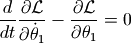
對于變量 $\theta_1$ 的拉格朗日方程：

$\frac{d}{dt}\frac{\partial \mathcal{L}}{\partial \dot \theta_1} - \frac{\partial \mathcal{L}}{\partial \theta_1} = 0$

得到：

$L_1 [(m_1+m_2)L_1{\ddot \theta_1} + m_2 L_2 \cos(\theta_1 - \theta_2) {\ddot \theta_2} + m_2 L_2 \sin(\theta_1 - \theta_2) {\dot \theta_2}^2 + (m_1+m_2) g \sin(\theta_1)] = 0$

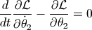
對于變量 $\theta_2$ 的拉格朗日方程：

$\frac{d}{dt}\frac{\partial \mathcal{L}}{\partial \dot \theta_2} - \frac{\partial \mathcal{L}}{\partial \theta_2} = 0$

得到：

$m_2 L_2 [L_2 {\ddot \theta_2} + L_1 \cos(\theta_1 - \theta_2) {\ddot \theta_1} - L_1 \sin(\theta_1 - \theta_2) {\dot \theta_1}^2 + g \sin(\theta_2)] = 0$

這一計算過程可以用sympy進行推導：

# -*- coding: utf-8 -*-
from sympy import *
from sympy import Derivative as D

var("x1 x2 y1 y2 l1 l2 m1 m2 th1 th2 dth1 dth2 ddth1 ddth2 t g tmp")

sublist = [
(D(th1(t), t, t), ddth1),
(D(th1(t), t), dth1),
(D(th2(t), t, t), ddth2),
(D(th2(t),t), dth2),
(th1(t), th1),
(th2(t), th2)    
]

x1 = l1*sin(th1(t))
y1 = -l1*cos(th1(t))
x2 = l1*sin(th1(t)) + l2*sin(th2(t))
y2 = -l1*cos(th1(t)) - l2*cos(th2(t))

vx1 = diff(x1, t)
vx2 = diff(x2, t)
vy1 = diff(y1, t)
vy2 = diff(y2, t)

# 拉格朗日量
L = m1/2*(vx1**2 + vy1**2) + m2/2*(vx2**2 + vy2**2) - m1*g*y1 - m2*g*y2

# 拉格朗日方程
def lagrange_equation(L, v):    
    a = L.subs(D(v(t), t), tmp).diff(tmp).subs(tmp, D(v(t), t))
    b = L.subs(D(v(t), t), tmp).subs(v(t), v).diff(v).subs(v, v(t)).subs(tmp, D(v(t), t))
    c = a.diff(t) - b
    c = c.subs(sublist)  
    c = trigsimp(simplify(c))
    c = collect(c, [th1,th2,dth1,dth2,ddth1,ddth2])
    return c

eq1 = lagrange_equation(L, th1)
eq2 = lagrange_equation(L, th2)

執行此程序之后，eq1對應于 $\theta_1$ 的拉格朗日方程， eq2對應于 $\theta_2$ 的方程。

由于sympy只能對符號變量求導數，即只能計算 D(L, t), 而不能計算D(f, v(t))。因此在求偏導數之前，將偏導數變量置換為一個tmp變量，然后對tmp變量求導數，例如下面的程序行對D(v(t), t)求偏導數，即計算 $\partial \mathcal{L} / \partial \dot v$

L.subs(D(v(t), t), tmp).diff(tmp).subs(tmp, D(v(t), t))

而在計算 $\partial \mathcal{L} / \partial v$ 時，需要將v(t)替換為v之后再進行微分計算。由于將v(t)替換為v的同時，會將 D(v(t), t) 中的也進行替換，這是我們不希望的結果，因此先將 D(v(t), t) 替換為tmp，微分計算完畢之后再替換回去：

L.subs(D(v(t), t), tmp).subs(v(t), v).diff(v).subs(v, v(t)).subs(tmp, D(v(t), t))

最后得到的eq1, eq2的值為：

>>> eq1
ddth1*(m1*l1**2 + m2*l1**2) +
ddth2*(l1*l2*m2*cos(th1)*cos(th2) + l1*l2*m2*sin(th1)*sin(th2)) +
dth2**2*(l1*l2*m2*cos(th2)*sin(th1) - l1*l2*m2*cos(th1)*sin(th2)) +
g*l1*m1*sin(th1) + g*l1*m2*sin(th1)
>>> eq2
ddth1*(l1*l2*m2*cos(th1)*cos(th2) + l1*l2*m2*sin(th1)*sin(th2)) +
dth1**2*(l1*l2*m2*cos(th1)*sin(th2) - l1*l2*m2*cos(th2)*sin(th1)) +
g*l2*m2*sin(th2) + ddth2*m2*l2**2

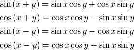
結果看上去挺復雜，其實只要運用如下的三角公式就和前面的結果一致了：

$\sin \left(x+y\right)=\sin x \cos y + \cos x \sin y \cos \left(x+y\right)=\cos x \cos y - \sin x \sin y \sin \left(x-y\right)=\sin x \cos y - \cos x \sin y \cos \left(x-y\right)=\cos x \cos y + \sin x \sin y$

微分方程的數值解?

接下來要做的事情就是對如下的微分方程求數值解：

$(m_1+m_2)L_1{\ddot \theta_1} + m_2 L_2 \cos(\theta_1 - \theta_2) {\ddot \theta_2} + m_2 L_2 \sin(\theta_1 - \theta_2) {\dot \theta_2}^2 + (m_1+m_2) g \sin(\theta_1) = 0$

$L_2 {\ddot \theta_2} + L_1 \cos(\theta_1 - \theta_2) {\ddot \theta_1} - L_1 \sin(\theta_1 - \theta_2) {\dot \theta_1}^2 + g \sin(\theta_2) = 0$

由于方程中包含二階導數，因此無法直接使用odeint函數進行數值求解，我們很容易將其改寫為4個一階微分方程組，4個未知變量為： $\theta_1, \theta_2, v_1, v_2$ ，其中 $v_1, v_2$ 為兩個桿轉動的角速度。

$\dot \theta_1 = v_1$

$\dot \theta_2 = v_2$

$(m_1+m_2)L_1{\dot v_1} + m_2 L_2 \cos(\theta_1 - \theta_2) {\dot v_2} + m_2 L_2 \sin(\theta_1 - \theta_2) {\dot \theta_2}^2 + (m_1+m_2) g \sin(\theta_1) = 0$

$L_2 {\dot v_2} + L_1 \cos(\theta_1 - \theta_2) {\dot v_1} - L_1 \sin(\theta_1 - \theta_2) {\dot \theta_1}^2 + g \sin(\theta_2) = 0$

下面的程序利用 scipy.integrate.odeint 對此微分方程組進行數值求解：

# -*- coding: utf-8 -*-

from math import sin,cos
import numpy as np
from scipy.integrate import odeint

g = 9.8

class DoublePendulum(object):
    def __init__(self, m1, m2, l1, l2):
        self.m1, self.m2, self.l1, self.l2 = m1, m2, l1, l2
        self.init_status = np.array([0.0,0.0,0.0,0.0])
        
    def equations(self, w, t):
        """
        微分方程公式
        """
        m1, m2, l1, l2 = self.m1, self.m2, self.l1, self.l2
        th1, th2, v1, v2 = w
        dth1 = v1
        dth2 = v2
        
        #eq of th1
        a = l1*l1*(m1+m2)  # dv1 parameter
        b = l1*m2*l2*cos(th1-th2) # dv2 paramter
        c = l1*(m2*l2*sin(th1-th2)*dth2*dth2 + (m1+m2)*g*sin(th1))
        
        #eq of th2
        d = m2*l2*l1*cos(th1-th2) # dv1 parameter
        e = m2*l2*l2 # dv2 parameter
        f = m2*l2*(-l1*sin(th1-th2)*dth1*dth1 + g*sin(th2))
        
        dv1, dv2 = np.linalg.solve([[a,b],[d,e]], [-c,-f])
        
        return np.array([dth1, dth2, dv1, dv2])
        
def double_pendulum_odeint(pendulum, ts, te, tstep):
    """
    對雙擺系統的微分方程組進行數值求解，返回兩個小球的X-Y坐標
    """
    t = np.arange(ts, te, tstep)
    track = odeint(pendulum.equations, pendulum.init_status, t)
    th1_array, th2_array = track[:,0], track[:, 1]
    l1, l2 = pendulum.l1, pendulum.l2
    x1 = l1*np.sin(th1_array)
    y1 = -l1*np.cos(th1_array)
    x2 = x1 + l2*np.sin(th2_array)
    y2 = y1 - l2*np.cos(th2_array)
    pendulum.init_status = track[-1,:].copy() #將最后的狀態賦給pendulum
    return [x1, y1, x2, y2]

if __name__ == "__main__":    
    import matplotlib.pyplot as pl
    pendulum = DoublePendulum(1.0, 2.0, 1.0, 2.0) 
    th1, th2 = 1.0, 2.0
    pendulum.init_status[:2] = th1, th2
    x1, y1, x2, y2 = double_pendulum_odeint(pendulum, 0, 30, 0.02)
    pl.plot(x1,y1, label = u"上球")
    pl.plot(x2,y2, label = u"下球")
    pl.title(u"雙擺系統的軌跡, 初始角度=%s,%s" % (th1, th2))
    pl.legend()
    pl.axis("equal")
    pl.show()

程序中的 DoublePendulum.equations 函數計算各個未知函數的導數，其輸入參數w數組中的變量依次為：

th1: 上球角度
th2: 下球角度
v1: 上球角速度
v2: 下球角速度

返回值為每個變量的導數：

dth1: 上球角速度
dth2: 下球角速度
dv1: 上球角加速度
dv2: 下球角加速度

其中dth1和dth2很容易計算，它們直接等于傳入的角速度變量：

dth1 = v1
dth2 = v2

為了計算dv1和dv2，需要將微分方程組進行變形為如下格式 :

$\dot v_1 = ... \dot v_2 = ...$

如果我們希望讓程序做這個事情的話，可以計算出 dv1 和 dv2 的系數，然后調用 linalg.solve 求解線型方程組：

#eq of th1
a = l1*l1*(m1+m2)  # dv1 parameter
b = l1*m2*l2*cos(th1-th2) # dv2 paramter
c = l1*(m2*l2*sin(th1-th2)*dth2*dth2 + (m1+m2)*g*sin(th1))

#eq of th2
d = m2*l2*l1*cos(th1-th2) # dv1 parameter
e = m2*l2*l2 # dv2 parameter
f = m2*l2*(-l1*sin(th1-th2)*dth1*dth1 + g*sin(th2))

dv1, dv2 = np.linalg.solve([[a,b],[d,e]], [-c,-f])

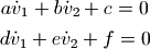
上面的程序相當于將原始的微分方程組變換為

$a \dot v_1 + b \dot v_2 + c = 0 d \dot v_1 + e \dot v_2 + f = 0$

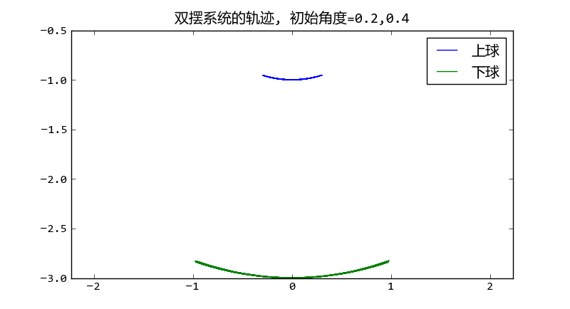
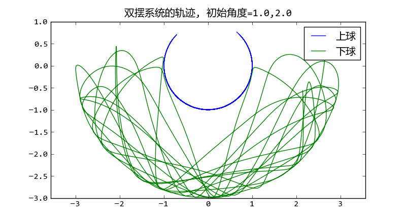
程序繪制的小球運動軌跡如下：

初始角度微小時的雙擺的擺動軌跡

大初始角度時雙擺的擺動軌跡呈現混沌現象

可以看出當初始角度很大的時候，擺動出現混沌現象。

動畫顯示?

計算出小球的軌跡之后我們很容易將結果可視化，制作成動畫效果。制作動畫可以有多種選擇：

visual庫可以制作3D動畫
pygame制作快速的2D動畫
tkinter或者wxpython直接在界面上繪制動畫

這里介紹如何使用matplotlib制作動畫。整個動畫繪制程序如下：

# -*- coding: utf-8 -*-
import matplotlib
matplotlib.use('WXAgg') # do this before importing pylab
import matplotlib.pyplot as pl
from double_pendulum_odeint import double_pendulum_odeint, DoublePendulum

fig = pl.figure(figsize=(4,4))
line1, = pl.plot([0,0], [0,0], "-o")
line2, = pl.plot([0,0], [0,0], "-o")
pl.axis("equal")
pl.xlim(-4,4)
pl.ylim(-4,2)

pendulum = DoublePendulum(1.0, 2.0, 1.0, 2.0)
pendulum.init_status[:] = 1.0, 2.0, 0, 0

x1, y1, x2, y2 = [],[],[],[]
idx = 0

def update_line(event):
    global x1, x2, y1, y2, idx
    if idx == len(x1):
        x1, y1, x2, y2 = double_pendulum_odeint(pendulum, 0, 1, 0.05)
        idx = 0 
    line1.set_xdata([0, x1[idx]])
    line1.set_ydata([0, y1[idx]])
    line2.set_xdata([x1[idx], x2[idx]])
    line2.set_ydata([y1[idx], y2[idx]])
    fig.canvas.draw()                 
    idx += 1

import wx
id = wx.NewId()
actor = fig.canvas.manager.frame
timer = wx.Timer(actor, id=id)
timer.Start(1)
wx.EVT_TIMER(actor, id, update_line)
pl.show()

程序中強制使用WXAgg進行后臺繪制：

matplotlib.use('WXAgg')

然后啟動wx庫中的時間事件調用update_line函數重新設置兩條直線的端點位置：

import wx
id = wx.NewId()
actor = fig.canvas.manager.frame
timer = wx.Timer(actor, id=id)
timer.Start(1)
wx.EVT_TIMER(actor, id, update_line)

在update_line函數中，每次軌跡數組播放完畢之后，就調用：

if idx == len(x1):
    x1, y1, x2, y2 = double_pendulum_odeint(pendulum, 0, 1, 0.05)
    idx = 0

重新生成下一秒鐘的軌跡。由于在 double_pendulum_odeint 函數中會將odeint計算的最終的狀態賦給 pendulum.init_status ，因此連續調用 double_pendulum_odeint 函數可以生成連續的運動軌跡

def double_pendulum_odeint(pendulum, ts, te, tstep):
    ...
    track = odeint(pendulum.equations, pendulum.init_status, t)
    ...
    pendulum.init_status = track[-1,:].copy()
    return [x1, y1, x2, y2]

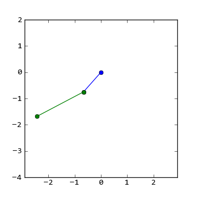
程序的動畫效果如下圖所示：

雙擺的擺動動畫效果截圖

單擺和雙擺模擬?

單擺模擬?

計算擺動周期?

雙擺模擬?

公式推導?

微分方程的數值解?

動畫顯示?

首頁目錄

上一篇文章

下一篇文章

Navigation

單擺和雙擺模擬?

單擺模擬?

計算擺動周期?

雙擺模擬?

公式推導?

微分方程的數值解?

動畫顯示?

首頁目錄

上一篇文章

下一篇文章

快速搜索

Navigation